Here, I’ll talk about regularized linear regression (aka Tikhonov regularization) and normal equations. I used regularization for my research to increase learning rate of ambient occlusion (AO) of skinned characters. Before directly diving into regularization, I’ll first talk about linear regression.
- Linear Regression and Gradient Descent
- Regularization
- Regularization with Normal Equation
- References
Linear Regression and Gradient Descent
Regression analysis can be simply explained as making connections among the variables. It helps us to understand how the value of the dependent variable changes when the independent variables is varied.
Let’s talk about one of the famous examples on the net: Deciding house price by learning house size. In this example, you simply train your system by house size-corresponding price training data, and then in the future estimate price of any houses by simply using their size.
Of course, you will not use some kind of black magic for doing this. You will use a simple linear function such as hθ(x) = θ0 + θ1x. Here, you can think that x is the size of the house (variable), hθ(x) is the price you estimated, and θs are the “magical” parameters you have learned using your training data. Actually, all we need and all we want are approximating these θs for estimation process.
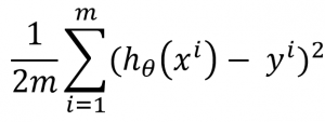
For getting the best parameters (θs), we should “minimize the cost function”. The cost function is the fancy way to say “use kinda MSE to check whether your estimation is close enough to the ground truth (y in the Equation 1)”. So, we will calculate (hθ(x) – y)2 for every sample in our data, and then sum the results, and then divide 2m, where m is the number of samples in the training data.
Before we start to talk about how to minimize the cost function, I’d suggest to talk about linear regression with multiple features. If you remember “approximating house price” example, we associated house price with only the size. But, this time we will also add features such as number of rooms, age of house, distance to bus stop. This will increase the realism, and the number of parameters we need to find out.
But don’t worry, working with multiple features actually will only add more addition to our hypothesis (hθ(x)). For example, if we use 4 features (size, number of rooms, age, distance to bus stop), our linear function will become hθ(x) = θ0x0 + θ1x1 + θ2x2 + θ3x3 + θ4x4. And as you can see this won’t change our cost function since hθ(x) still returns a scalar value.
Now, we can talk about how to minimize our cost function to adjust our parameters. For this task, first, we will talk about the famous gradient descent algorithm. Gradients act like a compass and always point the direction of local minimum. In this way, gradient descent algorithm reaches the local minimum by taking small steps. This algorithm starts with an initial guess, and performs minimization by adjusting the guess. But, before running the algorithm, first, we need to get the gradients by differentiating (derivative) the cost function.
When we take the derivative of the cost function we get the equation below:
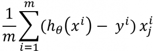
Here, m is number of samples, hθ(xi) is approximated value of the ith sample (for example, approximated price of the first house), yi is ground truth value for ith sample (real price of the first house), and xij is value of feature j for the ith sample (number of the rooms for the first house).
Gradient descent algorithm has two important things that can affect the results you get. The first one is the initial guess (First values we assign to θs). Different initial guesses lead you different local minimums. The second one, size of the step you are taking (learning rate (α)). If you take big steps, you may miss the local minimum. If you take small steps, it may take forever to reach the local minimum. And also, as you can guess, there are no magical numbers that can work with any types of data. So, you need to choose your own learning rate and initial guess.
Now, it’s time putting all together and give you the whole algorithm. But I have to tell you, the algorithm isn’t that complicated. Actually, it only contains one mathematical expression, and loops:
|
1 2 3 4 5 6 7 8 9 10 11 12 13 14 |
<strong>Gradient Descent Algorithm:</strong> for until we reach local minimum for each samples in the training data (index <em><strong>i</strong></em>) for each parameter (θs) (index <em><strong>j</strong></em>) Calculate learning rate (α) times the partial derivative of of the θ vector with respect to θj Update θj's value by subtracting the the result from old value of θj (Equation 3) end end end |
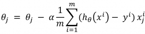
End the expression you will perform in the inner loop is
There is also another method you can use for linear regression problem. It’s called normal equation. The advantage of this method, it eliminates learning rate (α) and solves optimum value of θ analytically (No need to choose learning rate, no iteration to get a solution, the results are directly optimal). The disadvantage, it requires matrix operations (transpose, multiplication, and inverse) having high complexity.
I will talk about normal equation in regularization part.
If your system is working with many parameters, this possibly causes the problem called overfitting. In this case, the system gets confused and begins to make wrong decisions. For example, for the system I used to approximate AO values, I was working with around 48 000 parameters, and for complex motions (animations), approximation results were pretty inaccurate.
For solving the overfitting problem, we use regularization. Regularization helps us to simplify our hypothesis by penalizing some of the parameters. In this way, we reduce the effects of some parameters, and save our system to get confused.
So, if we add regularization term to our cost function (Equation 1), we get the equation below:
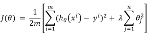
Here, λ is regularization parameter, and n is the number of parameters we have (In AO example, n equals to 48 000). Choosing the value of the regularization parameter (λ) is problematic and important. If you choose λ so small, it does not change anything. If you choose λ so large, you penalize all parameters and end up with underfitting.
If you don’t want to read papers about choosing the value of λ, generally values like 0.001 or 0.01 work well for it. So, I suggest you to start at something like 0.01, go down to something like 0.001, and also up something like 0.1, and check the approximations you get. This’ll give you some clues.
Regularized linear regression is also not much different than linear regression. You will use the derivative of the new cost function (Equation 4) for adjusting your parameters. You, you will only change the expression in the gradient descent algorithm:
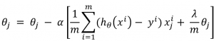
P.S. You can group θj terms in Equation 5, and make it better.
Regularization with Normal Equation
As I mentioned earlier, you can also use normal equation for the same task. In this case, you will use variable matrix (xs in the equations, the size of the house, number of rooms, age, etc.) and ground truth matrix (ys in the equations, the real price of the each house) to approximate parameter matrix (θs).
With this approach, you won’t need to concern about the learning rate (α) and you will get all optimal θs in a big matrix for each variable (xs):
![]()
So, in here T means transpose of the matrix, -1 is the inverse of the matrix, Θ contains all parameters we need for approximation process, X contains all variables affecting our approximation, λ is regularization parameter,Y contains all ground truth values, and M is the identity matrix with zero in the first diagonal element:
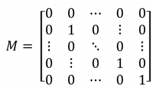
For example, if we are approximate per-vertex ambient occlusion (AO), each column of Θ contains all the parameters of a vertex, X contains joint angles or vertex positions, and Y contains ray-traced AO values.