This is the ray tracer I developed based on Nori for IFT 6095 Sujet en infographie/Real-time Rendering course. You can reach the source code on my GitHub page.
I implemented sphere, ray-sphere intersection, directional light, diffuse shading with hard shadows, anti-aliasing with super sampling, Monte Carlo integrator, implicit path tracing with biased path-length termination, explicit path tracing with Russian roulette.
In the future I am planing to continue by adding Phong shading, multiple importance sampling, environmental mapping, and volume rendering.
- Picking a Point on the Sphere
- Calculating Normal of a Point on the Sphere
- Ray-Sphere Intersection
- Diffuse Shading
- Anti-aliasing
- Monte Carlo Estimation
- Path Tracing
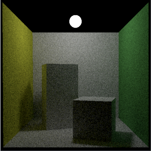
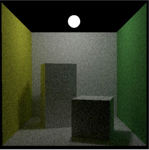
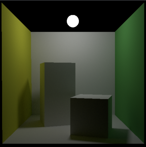
- Some of the Results
- References
Picking a Point on the Sphere
For the calculation, Global Illumination Compendium is referenced.
For picking a point on the sphere, the formula below is used
|
1 2 3 |
x = Cx + ( 2r * cos(2*PI*u1) * sqrt( u2(1-u2) ) y = Cy + ( 2r * sin(2*PI*u1) * sqrt( u2(1-u2) ) z = Cz + r(1 - 2u2) |
where Cx,y,z is the center of sphere, r is radius of the sphere, and u1,2 are random points.
Calculating Normal of a Point on the Sphere
For the calculation, formula from SIGGRAPH tutorial is used.
|
1 |
SN = [(xi - xc)/Sr, (yi - yc)/Sr, (zi - zc)/Sr] |
Where, SN is the surface normal, Xi, Yi, Zi are given point coordinates, Xc, Yc, Zc are coordinates of the sphere’s center.
For ray-sphere intersection, the algebraic method told in Ray-Sphere Intersection, SIGGRAPH Tutorial is used.
Algorithm
- Calculate A value: A = Xd^2 + Yd^2 + Zd^2 where Xd, Yd, and Zd are direction of the Ray
- Calculate B value: B = 2 * (Xd * (X0 – Xc) + Yd * (Y0 – Yc) + Zd * (Z0 – Zc)) where X0, Y0, Z0 are origin of the ray, and Xc, Yc, Zc are center of the sphere
- Calculate C value: C = (X0 – Xc)^2 + (Y0 – Yc)^2 + (Z0 – Zc)^2 – Sr^2 where Sr is radius of the sphere
- Calculate discriminant
- if(disc < 0.f), No intersection, return false.
- Calculate the first root: t0 = ( -b – sqrtDisc ) / (2*a)
- if t0 >= 0, there is no need to calculate t1. Because t0 will be the smallest root. Else calculate t1 = ( -b + sqrtDisc ) / (2*a)
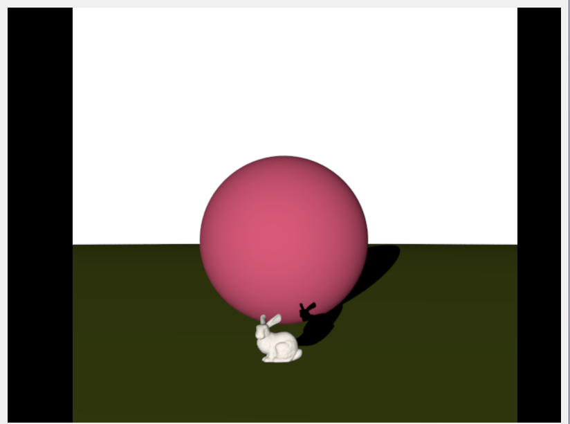
For calculating diffuse shading the formula below is used:
|
1 |
I = IaKa + IpKd(N dot L) |
Here, I stands for intensity (color) of the pixel, Ia for ambient
intensity and Ka for ambient coefficient. IaKa together defines
ambient color.
Ip stands for intensity of the light source and Kd for diffuse
reflection coeffient of the object.
(N dot L) defines dot product between surface normal (N) and light
direction vector (L). The result is the cosine value (angle) between
these two vectors.
IpKd(N dot L) stands for diffuse color.
Algorithm
- Check for the intersection. If there is no intersection, return background color.
- If there is an intersection, create a shadow ray as the origin is the intersection point, and the direction is the light direction.
- If the shadow ray hits an object, return ambient color.
- If the object is not in the shadow, calculate and return diffuse color of the pixel.
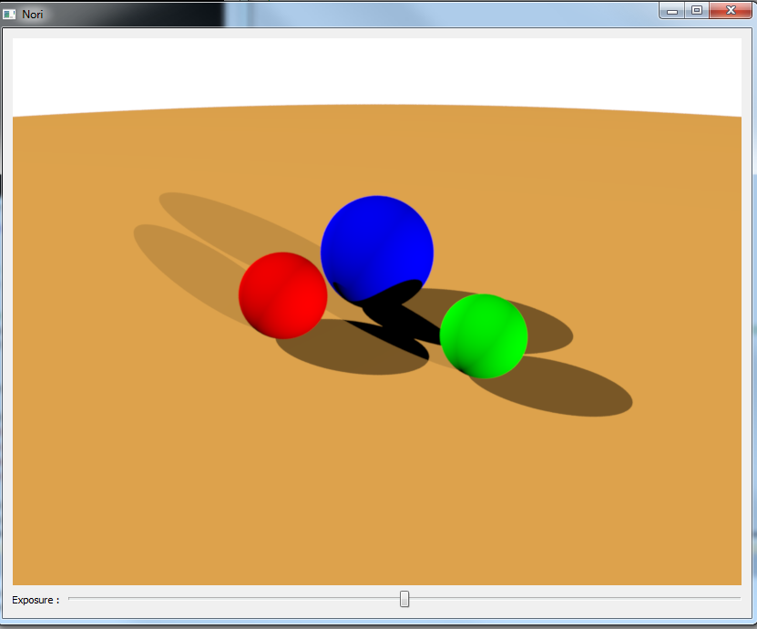
For anti-aliasing, uniform and stochastic super sampling approaches are used.
Uniform super sampling anti-aliasing was implemented with 5 (including the main ray) rays. For each pixel, one ray for each corner of the pixel, and a ray for the center are shot.
For stochastic super sampling, any number of rays are shot to the pixel in a random fashion (with random positions).
After each ray’s result is calculated, all results are summed and divided by the number of rays for calculating final color of the pixel.
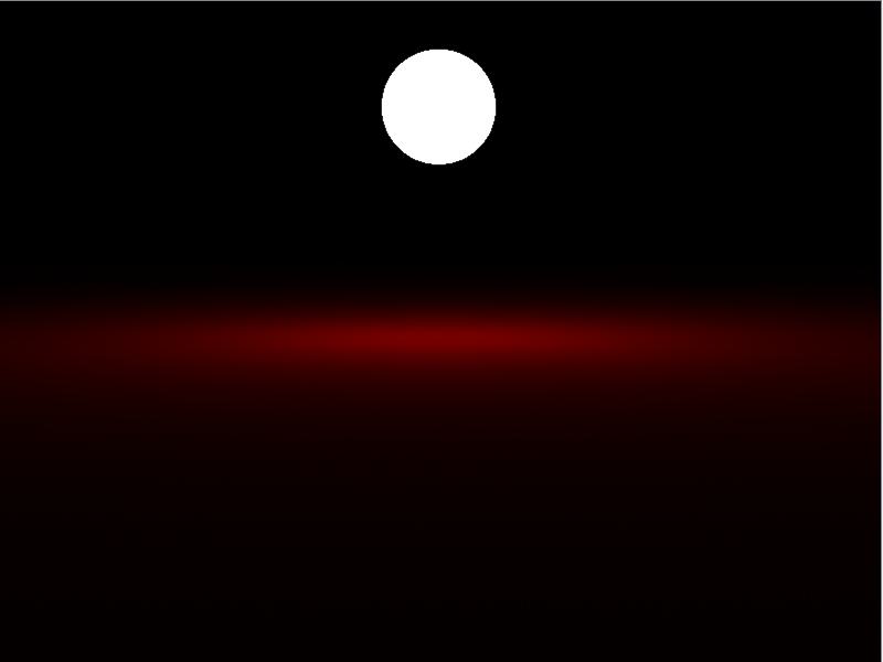
Normal ray tracing procedure is followed until an intersection is found. After finding one, if there is no intersection, background color is returned. Light color is returned if the object, which is hit by the ray, is a light source. Otherwise, the result is calculated by MC integrator. Shadow rays, and visibility is handled during the MC process.
f(x) was selected as diffuse shading formula which is Li * BRDF * n dot w. Here, Li is intensity of light, BRDF is diffuse color of the object, which is rho/PI, and n dot w is the angle between the surface normal, and light direction.
pdf(x) is selected differently for each type of MC integration.
Spherical MC Integration
Formula, which are used for generating random direction on unit sphere, are taken from PBRT 2nd Edition, CH 13 Monte Carlo Integration I: Basic Concepts page 664.
|
1 2 3 4 5 |
Direction.z = 1 - 2r1 Direction.x = sqrt(1 - Direction.z^2) * cos(2 * M_PI * r2) Direction.y = sqrt(1 - Direction.z^2) * sin(2 * M_PI * r2) <em>r1</em>, and <em>r2</em> are random values between 0 and 1. |
Because, uniform sphere sampling is used, pdf(x) is selected as 1 / 4*PI. Thus, final form of MC integration becomes 1/4*(Li * rho * n dot w).
Hemispherical MC Integration
Formula, which are used for generating random direction on unit hemisphere proportional to solid angle, are taken from Global Illumination Compendium.
|
1 2 3 4 5 |
Direction.x = cos(2*M_PI*r1) * sqrt(1 - r2^2) Direction.y = sin(2*M_PI*r1) * sqrt(1 - r2^2) Direction.z = r2 <em>r1</em>, and <em>r2</em> are random values between 0 and 1. |
Because, hemispherical sampling is used, pdf(x) is selected as 1/2*PI. Thus, final form of MC integration becomes 1/2*(Li * rho * n dot w)
Cosine-Weighted MC Integration
Formulae are taken from IFT 6095 slides to implement unit hemisphere proportional to cosine-weighted solid angle sampling. For direction picking, formula on Techniques: Illumination Globale slide (page 48), and for converting to Cartesian coordinates, formula on Théorie: Illumination Directe slide (page 39) are used.
|
1 2 3 4 5 6 7 8 |
float theta = acosf( sqrt(r1) ); float phi = 2 * M_PI * r2; Vector3f direction = Vector3f( sinf(theta) * cosf(phi), // X sinf(theta) * sinf(phi), // Y cosf(theta)); // Z <em>r1</em>, and <em>r2 </em>are random values between 0 and 1. |
Because, cosine-weighted sampling is used, pdf(x) is selected as ndotW/PI. Thus, final form of MC integration becomes (Li * rho).
Surface Area Sampling
For Spherical Surface Area calculations formula, Global Illumination Compendium is used.
For picking a point on the sphere:
|
1 2 3 4 5 6 7 8 9 10 11 |
Picking a point on the sphere (selectedPoint): x = Cx + ( 2r * cos(2*PI*u1) * sqrt( u2(1-u2) ) y = Cy + ( 2r * sin(2*PI*u1) * sqrt( u2(1-u2) ) z = Cz + r(1 - 2u2) where <em>Cx,y,z</em> is the center of sphere, <em>r</em> is radius of the sphere, and <em>u1,2</em> are random points. Getting the direction (in world coordinates): direction = selectedPoint - firstIntersectionPoint |
pdf(x) = 1 / 4*PI*r^2 where r is radius of the sphere (1 / Surface area of sphere)
f(x) = Li * BRDF(P/M_PI) * n dot W * nL dot WL) / PDF * d^2 ] where nL dot wL is the angle between the selected direction, and light source normal, and d^2 is the distance between intersection point, and selected point on the light.
Importance Sampling According to Solid Angle
For coding spherical light importance sampling implementation according to solid angle, PBRT 2nd edition book, Section 14.6 Sampling Light Sources [720,722] pages, and PBRT v2 source code are referenced.
Algortihm
- Get direction: Needs random values, center of the sphere (light), normal at the intersection point, cosThetamax (needs radius of the sphere (light), and the coordinate system (needs vector between intersection point, and center of the sphere (light) for aligning the cone with the light)
- Sample the ray
- Calculate visibility
- Calculate contrution Li * brdf * cosTheta / pdf(x)
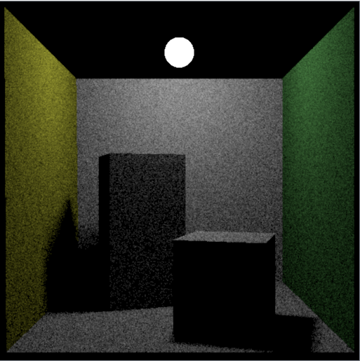
Implicit path tracing with uniform solid angle sampling and biased path-length termination: Follow normal ray tracing procedure until finding an intersection. If there is no intersection, return background color. If the object is light, directly return light color. Otherwise, call path tracing integrator, and return calculated result. Shadow rays, and checking whether the object in shadow or not will be handle during the MC process.
Algorithm:
- Pick a direction from the point by using unit sphere sampling
- Calculate contribution at the point P
- Shoot the ray
- If the ray hits the light, returns Le value of the light. If the ray hits another object, call yourself from the latest point you hit by increasing the path length. If there is no intersection (which means ray goes out of the scene), return background color
Explicit path tracing with surface area sampling, and Russian roulette path termination: Follow normal ray tracing procedure until finding an intersection. If there is no intersection, return background color. If the object is light, directly return light color. Otherwise, call path tracing integrator, and return calculated result. Shadow rays, and checking whether the object in shadow or not will be handle during the MC process.
Algorithm
- Calculate light contribution by surface area sampling (Don’t forget to check visibility of the selected point on the sphere)
- Check for the path length termination
- If there is no reason to terminate, calculate contribution of this point.
- Pick a direction by using cosine-weighted sampling for the next point of the path, and shoot the ray
- If the ray hits the light, returns color. If the ray hits another object, call yourself from the latest point you hit.